The goal of this blogpost is to explain quantum capacity theorem and its proofs (achievability and converse). First, we shall build our intuition through a toy example of private classical communication and creation of one distance-separated shared entanglement using a specific noisy quantum channel. Finally, we shall dive into the statement and proofs of quantum capacity theorem.

Prerequisites: Classical information theory : asymptotic equipartition property and Shannon’s channel coding theorem; Quantum information processing: superposition, entanglement, density matrix formalism.

Transmitting Quantum Information

The operational meaning of classical capacity is the maximum rate of transmission of classical information in bits per “channel use” over a noisy channel. But, what does it mean to communicate quantum information? It is possible to send bit strings, product states, or entangled states over quantum channels, therefore we need a more precise definition of quantum communication. The operational meaning of quantum communication is the rate at which one can transmit entanglement over many uses of noisy quantum channels. Precisely, it quantifies the number of qubits, one from each entangled pair, that can be transmitted reliably for each “use” of the quantum channel to create shared entangled pairs over long distances.

In classical information theory, Claude E. Shannon single-handedly defined mutual information and proved the channel capacity theorem. This was not the case for quantum capacity theorem. The term quantum capacity was first introduced in a seminal paper by Peter Shor on quantum error correction in 1995. Subsequent papers over a span of 5 years refined the definition of quantum information and proofs of achievability and converses of quantum channel capacity theorem. In this blog, we shall review the sketch of the proof from the paper On quantum fidelities and channel capacities by Barnum et al in 2000.

Example 1: Private Classical Communication

First, let us demonstrate with the help of a toy example the private classical communication between Alice and Bob even though Eve can partially eavesdrop (the original term for this was secrecy capacity of a wiretap channel). The intuition developed here, will help later in understanding quantum capacity theorem. Suppose Alice can reliably transmit 00, 01, 10, 11 to Bob, which amounts to 2 bits of information. Suppose, Eve can learn about the 2nd bit and learn one-half of what is being communicated. Now, to privately communicate, Alice should not transmit any information on the 2nd bit. Now suppose Alice has a bit string (information) $m_1, m_2, …$ that she wants to transmit, if $m_i$ = 0, transmit 00 or 01 (channel symbols) at uniformly random, on the other hand, if $m_i$ = 1, then transmit 10 or 11 uniformly at random to Bob. In other words, Alice has to randomize over 2nd bit. The following color-coded table shows the bit pairs indexed by message (m) and randomizing variable (k). Consequently, Alice can only send 1 bit of private information to Bob. In general, if the (classical) mutual information between A and B is $I(A;B)$ and that between A and E is $I(A;B)$, then the number of distinguishable codewords Alice can send privately to Bob is $2^{n(I(A;B) - I(A;E))}$, which implies that the private classical information = $I(A;B) - I(A;E)$ (A. D. Wyner, 1975). In this example, $I(A;B)$=2 bits and $I(A;E)$=1 bit.

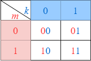
Figure 1. Table entries are the codewords of Alice. m is the message dimension, k is the randomization variable. Each codeword is indexed by the pair (m, k).

Example 2: Creating one shared entanglement

Now we shall use the idea of private classical communication to transmit one qubit of an entangled pair from Alice to Bob. This example would later help in appreciating the intuition behind the general case considered in the achievability proof.

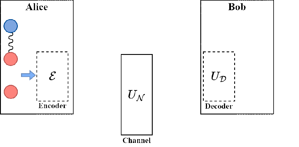Figure 2: Creating one shared entanglement between Alice and Bob, by Alice transmitting one share of her qubits over a noisy quantum channel by quantum channel coding such that the Bob receives the qubit reliably.

Suppose Alice has an entangled state $ \vert \psi\rangle_{RA}$, here the subscripts denote two quantum systems R and A (Reference and Alice, respectively). Here assume both R and A are Alice’s systems, have the same dimensions, and are entangled with each other. Consider an example entangled state $\left( a \vert 00\rangle + b \vert 11\rangle \right)$. The entanglement between R and A are indicated by the squiggly line between first and second qubit (counting from top to bottom) in the animation above. With a goal of creating shared entanglement with Bob, Alice decides to send qubit A to Bob. First, she encodes the qubit A as: $ \vert 0\rangle \rightarrow \frac{1}{\sqrt{2}} \left( \vert 00\rangle + \vert 01\rangle \right)$ and $ \vert 1\rangle \rightarrow \frac{1}{\sqrt{2}} \left( \vert 10\rangle + \vert 11\rangle \right)$. This encoding is chosen because as we will see later, the environment entangles with the second qubit (similar to the private communication in the classical case). Instead of randomly choosing one code word as in the classical case, we construct a uniform superposition over all codewords in the “randomization” set (across columns indexed by k in the previous subsection). Consequently, the state after encoding becomes:

$\left( a \vert 00\rangle + b \vert 11\rangle \right) \rightarrow \frac{a}{\sqrt{2}} \vert 0\rangle \otimes \left( \vert 00\rangle + \vert 01\rangle \right) + \frac{b}{\sqrt{2}} \vert 0\rangle \otimes \left( \vert 10\rangle + \vert 11\rangle \right)$.

Now, suppose the environment interacts (entangles) with the encoded qubits in the following manner:

$\frac{a}{\sqrt{2}} \vert 0\rangle \otimes \left( \vert 00\rangle + \vert 01\rangle \right) + \frac{b}{\sqrt{2}} \vert 0\rangle \otimes \left( \vert 10\rangle + \vert 11\rangle \right) \ \rightarrow \frac{a}{\sqrt{2}} \vert 0\rangle \otimes \left( \vert 00e_0\rangle + \vert 01e_1\rangle \right) + \frac{b}{\sqrt{2}} \vert 0\rangle \otimes \left( \vert 10e_0\rangle - \vert 11e_1\rangle \right)$

where $e_0$ and $e_1$ are the orthogonal states of the environment. In this channel model, the environment entangles with the second encoded qubit (similar to the private classical information case) and adds a phase of $\pi$ (negative sign) when both the encoded qubits are 11 (the last superposition state of the encoded qubits in the expression above).

Finally, Bob applies a unitary transformation or a decoding operation (a controlled-Z gate in this example) to only the encoded qubits (2nd and 3rd qubit) to obtain the following product state:

$\left( a \vert 00\rangle + b \vert 11\rangle \right) \otimes \frac{1}{\sqrt{2}} \left( \vert 0e_0\rangle + \vert 1e_1\rangle \right)$.

Note that the decoder decouples the qubits as follows: Bob’s first qubit is entangled with Alice’s qubit R, and Bob’s 2nd qubit is entangled with the environment, and these entangled pairs are independent. In other words, the entanglement with the environment is restricted only to Bob’s 2nd qubit which can be discarded, which is the main reason for using redundant qubits. At the end of this procedure, Alice and Bob share one pair of distance-separated entanglement, which was our primary goal. In the next section, we shall go through the achievability proof which will be a generalized version of this toy example.

Quantum Capacity Theorem

Statement

The quantum capacity of a quantum channel $\mathcal{N}$ is $\mathcal{Q}(\mathcal{N}) = \max~I(A \rangle B)$, where $I(A \rangle B)$ is the coherent information from A to B.

Achievability

The proof of achievability (direct coding) uses typicality arguments similar to that of the classical channel coding theorem. However, we need a slightly different notion of typicality in the quantum case. Please refer to [Mark Wilde’s textbook, Chapter 15] for a rigorous treatment of the quantum version of typicality.

In quantum information theory, instead of typical sets as in the classical case there is a notion of typical subspaces. This arises due to the superposition of quantum states. For example, suppose 0…000 and 1…111 belong to the typical set, there is no notion of superpositions in the classical case. On the other hand, in the quantum setting the uncountable set of all superpositions of $ \vert 0…000\rangle$ and $ \vert 1…111\rangle$ are also typical, which gives rise to the notion of a typical subspace (also referred to as coherent version or informally “coherification” of the classical code). Fortunately, in most cases, classical typicality arguments carry over directly to the quantum case, which helps in determining the dimensionality of the typical subspace and consequently, the rate of information transmission over quantum channels.

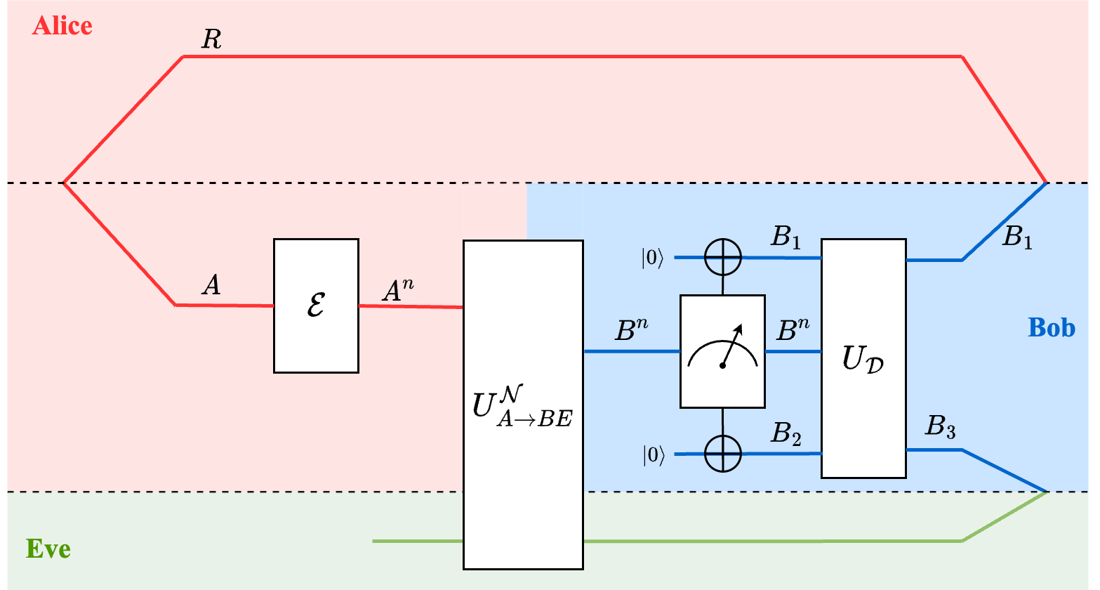Figure 3: Schematic of entanglement transmission over n-uses of the quantum channel. The quantum systems of Alice, Bob and Environment (Eve) are color-coded in red, blue, and green, respectively.

As we saw in the toy example (transmitting a single qubit in an entangled pair), the idea is to create codewords as a superposition of quantum states according to the “randomization” set such that the quantum state received by Eve is almost independent of the chosen message $m$.

The schematic of entanglement transmission including encoder, channel and decoder are shown in the Figure above. In our discussion, we shall focus more on intuition and will be slightly less rigorous than in the paper by Barnum et al and Mark Wilde’s textbook.

The basic idea of the proof of achievability follows by taking advantage of the private classical codes, i.e, choose codewords from the typical set as the basis for quantum code, and then “quantumify” the code (i.e., by considering its coherent version/superpositions of basis codewords), then prove systematically that at this rate, Bob can recover the state with high fidelity.

Consider a density matrix $\rho_A = \sum\limits_x p_X(x) \vert \psi_x\rangle \langle \psi_x \vert_A$. Let ${x^n(m, k)}_{m \in \mathcal{M}, k \in \mathcal{K}}$ be a random codebook constructed i.i.d. using the distribution $p_X(x)$. From private capacity conditions, for $n$ uses of the quantum channel, if $ \vert \mathcal{M} \vert \approx 2^{n[I(X ; B)-I(X ; E)]}$ and $ \vert \mathcal{K} \vert \approx 2^{n I(X ; E)}$, then the following conditions must hold.

1. \[\forall m \in \mathcal{M}, k \in \mathcal{K}: Tr\left\{\Lambda_{B^{n}}^{m, k} \rho_{B^{n}}^{x^{n}(m, k)}\right\} \geq 1-\varepsilon\]
2. \[\forall m \in \mathcal{M}:\vert \vert \frac{1}{ \vert \mathcal{K} \vert } \sum_{k \in \mathcal{K}} \omega_{E^{n}}^{x^{n}(m, k)}-\omega^{\otimes n} \vert \vert _{1} \leq \varepsilon\]

where $\omega \equiv \sum_{x} p_{X}(x) \omega_{E}^{x}$. The first condition indicates that if Alice encodes the message $(m, k)$ as $ \vert x^n(m, k)\rangle \langle x^n(m, k) \vert $, then the quantum state received by Bob $\rho_{B^{n}}^{x^{n}(m, k)}$ occupies a subspace that is almost disjoint from all other messages $(m’, k’) \neq (m, k)$, and $\Lambda_{B^{n}}^{m, k}$ is the typical subspace projector corresponding to the message $(m, k)$. Intuitively, comparison with the classical information theory gives the following equivalences: $\rho_{B^{n}}^{x^{n}(m, k)}$ is equivalent to the pmf $p(Y^n \vert X^n = x^n(m))$ and \(Tr\left\{\Lambda_{B^{n}}^{m, k} \rho_{B^{n}}^{x^{n}(m, k)}\right\}\) is equivalent to the conditional probability of successful decoding given message $m$, which is $\sum_{y^n: g(y^n) = m} p(y^n \vert x^n(m))$, where $g(\cdot)$ is the decoder. The second inequality indicates that what Eve (or the environment) receives is very close in fidelity to $\omega^{\otimes n}$, which means that Eve receives a quantum state almost independent of the message $m$.

In the quantum settting $I(X ; B)-I(X ; E)$ evaluates to the following:

$I(X ; B)-I(X ; E)=H(B)-H(E)=\text{H}(\text{B})-\text{H}(\text{AB})=\text{I}(\text{A} \rangle \text{B})$ = coherent information between Alice and Bob. Note that $\text{H}(\text{B})-\text{H}(\text{AB}) = -H(A \vert B)$ (negative of conditional entropy!!!). In classical information theory, every quantity of information is non-negative. However, in quantum information theory it is valid for conditional entropy can be negative, and the negative of conditional entropy is called coherent information.

Suppose Alice creates an entangled quantum state $ \vert \varphi\rangle_{R A} \equiv \sum\limits_m a_m \vert m\rangle_R \vert m\rangle_A$ in her lab (Alice has access to both the systems R and A). Suppose Alice wants to transmit her subsystem A to Bob. Then, the encoder $\mathcal{E}$ maps each $ \vert m\rangle_A$ in the superposition coherently to for a superposition of quantum codewords as follows:

$\mathcal{E}: \vert m\rangle_A \rightarrow \vert \phi_{m}\rangle_{A^{n}} \equiv \frac{1}{\sqrt{ \vert \mathcal{K} \vert }} \sum_{k \in \mathcal{K}} \vert \psi^{x^{n}(m, k)}\rangle_{A^{n}}$

where $A^n$ denotes $n^{th}$ extension of Alice’s subsytem A. Here $x^n$ is chosen from the typical set under the distribution $p_X(x)$, and $ \vert \psi^{x^{n}(m, k)}\rangle = \vert \psi^{x_0}\psi^{x_1} . . .\psi^{x_n}\rangle$. Moreover, note that instead of randomization over $k$, quantum codewords are uniform superposition over $k$, which can be interpreted as a quantum version of choosing codewords uniformly at random among $\mathcal{K}$ codewords. After encoding, the quantum state (of the joint system $R, A^n$) becomes:

$\sum_{m} \alpha_{m} \vert m\rangle_{R} \vert \phi_{m}\rangle_{A^{n}}$

Now, Alice sends the qubits of subsystem $A^n$ through $n$ instances of the (isometrically extended) channel $U_{A \rightarrow BE}$, resulting in the following state (notice the subscript of $\phi_{m}$):

$\sum_{m} \alpha_{m} \vert m\rangle_{R} \vert \phi_{m}\rangle_{B^nE^n}$

Now, at the receiver Bob has 3 subsystems - $B^n, B_1, B_2$. As we will see shortly, the idea is to recover the qubit sent by Alice in Bob’s subsystem $B_1$, which will be entangled with Alice’s subsystem $R$, and to trap the ‘noise’ introduced by the channel (interaction with the environment) in subsystem $B^n B_2$.

Bob creates a superposition $\sum_{m, k} \vert m\rangle \vert k\rangle$ in subsystems $B_1 B_2$ and then performs a coherent measurement on $B^n B_1 B_2$ such that each rotated codeword $ \vert \phi_{m}\rangle_{B^nE^n}$ (rotated by the channel) is almost uniquely entangled with $ \vert m \rangle \vert k \rangle$ using the subspace projector $\Lambda_{B^{n}}^{m, k}$, which yields the following state:

$\sum_{m} \sum_{k} \frac{1}{\sqrt{ \vert \mathcal{K} \vert }} \alpha_{m} \vert m\rangle_{R} \vert \psi^{x^n(m,k)}\rangle_{B^nE^n} \vert m\rangle_{B_1} \vert k\rangle_{B_2}$

In the Figure, this operation is shown by block with a meter symbol on $B^n$ connected to xor’s on $B_1$ and $B_2$.

Finally, there exists a controlled isometry $\sum\limits_{m} \vert m\rangle \langle m \vert_{B{1}} \otimes U_{B^{n} B_{2} \rightarrow B_{3}}^{m}$ such that signal and noise are decoupled. That the entanglement of the environment with Bob’s subsystems is restricted only to subsystem $B_3$, and the superposition of codewords is decoded (mapped) to superposition of messages in subsystem $B_1$.

$\left(\sum_{m \in \mathcal{M}} \alpha_{m} \vert m\rangle_{R} \vert m\rangle_{B_{1}}\right) \otimes \vert \theta\rangle_{B_{3}E^{n}}$

Now, Bob can discard subsystem $B_3$ and retain only $B_1$ which is entangled with Alice’s subsystem $R$ as expected. This completes the achievability proof.

Converse

Similar to Shannon’s channel coding theorem, the proof of converse of quantum capacity theorem is shorter. Suppose Alice has a pair of entangled qubits $\Phi_{RA}$, and she wants to send her subsystem A (one qubit from each pair) to Bob. Let \((\mathcal{E}_{A \rightarrow A^n}, \mathcal{D}_{B^n \rightarrow B})\) is an encoder decoder pair for the channel \(\mathcal{N}_{A^n \rightarrow B^n}\), then the received quantum state after Bob decodes is given by \(\omega_{RB} = \mathcal{D}_{B^n \rightarrow B} \circ \mathcal{N}_{A^n \rightarrow B^n} \circ \mathcal{E}_{A \rightarrow A^n}(\Phi_{RA})\). For the converse part we need to prove that if \(\frac{1}{2} \vert \vert \omega_{RB} - \Phi_{RA} \vert \vert <\epsilon\), then \(R = \frac{\log \vert A \vert }{n} \leq \mathcal{Q}(\mathcal{N})\).

In classical information theory, the main ingredients for the proof is Fano’s inequality and data processing inequalities. In quantum information theory, instead of Fano, another inequality called AFW (Alicki–Fannes–Winter) inequality is used for the proof (See QIT textbook, Theorem 11.10.3 for AFW inequality). Similar to Fano, the AFW inequality connects trace distance (error in classical) and entropy. The proof follows the following steps:

The first inequality is due to AFW inequality, the send inequality is due maximization of coherent information over $\omega$, and the last inequality is because of the definition of quantum capacity. Now, for a class of channels called degradable channels coherent information is additive. Restricting to only such channels, we obtain

\(R = \frac{\log \vert A \vert }{n}\leq Q(\mathcal{N})+ 2 \epsilon \frac{\log \vert A \vert }{n} + \frac{h_2(\epsilon)}{n}\).

Now, similar to classical converse, we can see that if $R>Q(\mathcal{N})$, then the trace distance (error in classical) is bounded away from 0. Therefore, \(R<Q(\mathcal{N})\) is a necessary condition for the trace distance to be bounded as \(\frac{1}{2} \vert \vert \omega_{RB} - \Phi_{RA} \vert \vert <\epsilon\) for any \(\epsilon \in (0, 1)\). This concludes the proof of converse part.